Overview of MPS Analysis

library(MPSurvey)

Walkthrough Overview

This walkthrough guides you through the analysis process for a 2022 mobile phone survey conducted in Rwanda. The data for the analysis and the questionnaire metadata can be accessed at the following links and saved on your computer:

The analysis follows the general structure outlined below:

Loading survey data and questionnaire metadata
Labeling and describing data, applying skip logic, and recoding indicators
Analyzing survey data
Exporting results and other outputs

Loading survey data and questionnaire metadata

The survey data can be loaded with read.csv("ug_publicuse_5421.csv"). Loading the questionnaire metadata relies on the following three functions: get_codebook(), get_descriptions(), and get_skiplogic(). The R code below shows these steps and their output:

Loading data

rw_publicuse_4483 <- read.csv("rw_publicuse_4483.csv")

Importing codebook

The codebook contains each variable (grp) and the potential response labels (values) and the responses coded in the data (options).

codebook <- get_codebook(path = "manifest.json")

Importing variable descriptions

The descriptions contains a detailed description (desc) for each variable (var).

descriptions <- get_descriptions(path = "manifest.json")

Importing skip logic

A data frame containing the skip logic information, including variables, question IDs, question text, response values, and skip logic conditions.

skip <- get_skiplogic(path = "manifest.json")

These inputs are used in data manipulation, analysis, and exporting functions and the above functions are frequently referenced within processing steps.

Labeling and describing data, applying skip logic, and recoding indicators

Label data

The first step in the data manipulation process is to apply data labels to the survey data using the output from get_codebook().

rw_label <- label_data(rw_publicuse_4483, codebook = codebook)

Applying skip logic

Following the labeling of data, skip logic from the questionnaire is applied to the survey results to determine when missing values are truly NA or if they should be recoded as NOT APPLICABLE. As this function runs, it will output information in the console that highlights the variable that previous responses could potentially skip (Skip Logic Variable) and the parent value and responses that would allow that variable to be shown to a respondent (Parent variable and Response values).

rw_label_skip <- apply_skiplogic(path = "manifest.json", x = rw_label)

#> 
#> 
#> ***** Skip Logic Variable: urbanicity *****
#> Parent variable: location
#> Response values: East
#>  Response values: West
#>  Response values: South
#>  Response values: North
#>  Response values: Skip
#>  Response values: City of Kigali
#> 
#> 
#> ***** Skip Logic Variable: education *****
#> Parent variable: urbanicity
#> Response values: City
#>  Response values: Rural
#>  Response values: Skip
#> 
#> 
#> ***** Skip Logic Variable: smoke1_daily *****
#> Parent variable: smoke1
#> Response values: Yes
#> 
#> 
#> ***** Skip Logic Variable: smoke1_ever *****
#> Parent variable: smoke1
#> Response values: No
#>  Response values: Skip
#> 
#> 
#> ***** Skip Logic Variable: smoke2 *****
#> 
#> 
#> ***** Skip Logic Variable: smoke1_everdaily *****
#> 
#> 
#> ***** Skip Logic Variable: smoke2_ever *****
#> Parent variable: smoke2
#> Response values: No
#>  Response values: Skip
#> 
#> 
#> ***** Skip Logic Variable: ets_home *****
#> 
#> 
#> ***** Skip Logic Variable: ets_work *****
#> Parent variable: ets_home
#> Response values: Yes
#>  Response values: No
#>  Response values: Skip
#> 
#> 
#> ***** Skip Logic Variable: alcohol_freq *****
#> Parent variable: alcohol_12mth
#> Response values: Yes
#> 
#> 
#> ***** Skip Logic Variable: alcohol1 *****
#> Parent variable: alcohol_freq
#> Response values: Daily
#>  Response values: 3-6 days per week
#>  Response values: 1-2 days per week
#>  Response values: 1-3 days per month
#>  Response values: Less than once per month
#>  Response values: Skip
#> 
#> 
#> ***** Skip Logic Variable: vegetable1 *****
#> 
#> 
#> ***** Skip Logic Variable: fruit2 *****
#> Parent variable: fruit1
#> Response values: from 1 to 7
#> Skip values:
#> 
#> 
#> ***** Skip Logic Variable: salt1 *****
#> 
#> 
#> ***** Skip Logic Variable: vegetable2 *****
#> Parent variable: vegetable1
#> Response values: from 1 to 7
#> Skip values:
#> 
#> 
#> ***** Skip Logic Variable: salt2 *****
#> Parent variable: salt1
#> Response values: Always
#>  Response values: Often
#>  Response values: Sometimes
#>  Response values: Rarely
#>  Response values: Never
#>  Response values: Skip
#> 
#> 
#> ***** Skip Logic Variable: salt3 *****
#> Parent variable: salt2
#> Response values: Always
#>  Response values: Often
#>  Response values: Sometimes
#>  Response values: Rarely
#>  Response values: Never
#>  Response values: Don't Know
#>  Response values: Skip
#> 
#> 
#> ***** Skip Logic Variable: bp1 *****
#> Parent variable: bp_measured
#> Response values: Yes
#> 
#> 
#> ***** Skip Logic Variable: bp2 *****
#> Parent variable: bp1
#> Response values: Yes

Recoding variables

Once skip logic is applied, we can then move into recoding variables or generating new variables to use in the analysis. One example is with smoke1 and smoke1_ever. smoke1 asks whether a respondent currently smokes tobacco products and smoke1_ever asks respondents if they have ever smoked tobacco products. Due to the built-in skip logic, if a person answered yes to smoke1, they wouldn’t be asked smoke1_ever because we know that they currently smoke tobacco products. To get the correct population-level indicator for smoke1_ever, we need to account for the yes’s from smoke1. To do this, we can use the recode_var() function.

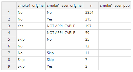
rw_analysis <- recode_var(rw_label_skip, vars=c("smoke1", "smoke1_ever"),new_var = smoke1_ever_pop)

Running this function will generate a popup window like the image below. This is where you can copy over the correct values for the new variable called smoke1_ever_pop.

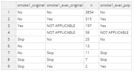
Applying the logic above, the completed table should look like the table below. Once complete, select ‘done’ at the top right and the edited dataset will be saved as rw_analysis.

The recode_var() function can be used for any new variables that need to be created. REMINDER: always write the output of this function back to the same analysis dataframe to save the edits.

Setting final descriptions

The final step is to set the final variable descriptions, especially for any newly developed indicators from the recode_var() function. The set_descriptions() function will also create a popup window where you can add or edit descriptions.

desc <- set_descriptions(path="manifest.json", x=rw_analysis)

Analyzing survey data

Selecting survey variables for analysis

The first step in this process is to select the variables of interest for the MPS analysis using the survey_variables() function. This function will create a popup window like the image below where you can toggle variables for inclusion in the analysis. Only select the indicator variables that will correspond to the population-level estimates and not the variables used for strata/weighting as those are selected in a different step.

vars <- survey_variables(desc = desc)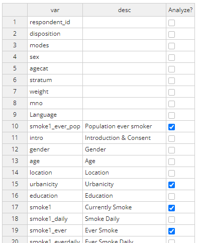

Creating survey design object

Once the variables are selected, we will use the mps_design() function to generate the survey design object using the srvyr package. This function requires the following information:

df: the analytic dataframe
ids: the unique identifiers for respondents, usually respondent_id
strata: the strata used for sampling and weighting, typically agecat and sex
weight: the variable storing the weighting value
vars: the list of variables for the analysis

mps <- mps_design(df = rw_analysis, 
                  ids = respondent_id, 
                  strata = c(agecat, sex), 
                  weight = weight, 
                  vars = vars)

The mps object is now a tbl_svy object that can be used for weighted survey analysis. The object has the following characteristics:

#> Stratified Independent Sampling design (with replacement)
#> Called via srvyr
#> Sampling variables:
#>   - ids: respondent_id 
#>   - strata: `agecat + sex` 
#>   - weights: weight 
#> Data variables: 
#>   - respondent_id (chr), agecat (chr), sex (chr), weight (dbl), urbanicity
#>     (chr), smoke1 (chr), smoke1_ever_pop (chr)

Calculating item non-response rates

When analyzing survey data, item non-response (INR) is an important factor in evaluating respondent interaction with the survey and responses for individual questions. The MPSurvey package has a function, get_inr() that calculates INR for selected variables from the survey_variables() function. Users can also choose to include_skips as valid responses by setting this value to TRUE although most situations should use the default value of FALSE.

inr <- get_inr(rw_analysis, vars=vars, include_skips = FALSE)

The output of this function is a list of two dataframes. The first, inr, contains one row for each variable of interest with the percent non-response (perc_non_response), the total number of valid responses (n_resp), and the total number of eligible respondents for the question (total). The second dataframe, responses, shows the total number of responses for each potential response option for all variables of interest.

Analyze survey

Analyzing the survey can be done using two functions: analyze_survey() and analyze_survey2(). The only difference between these is that analyze_survey() provides overall estimates and estimates by sex where analyze_survey2() provides overall estimates, estimates by sex, estimates by agecat, and estimates stratified by both sex and agecat.

NOTE: to use these functions, the dataframe must have variables names sex and agecat.

results <- analyze_survey(mps, vars=vars)
results2 <- analyze_survey2(mps, vars=vars)

The outputs of these functions are tbl_svysummary objects that render as formatted tables in the Viewer pane in RStudio.

results

Characteristic	Overall¹	95% CI	Female¹	95% CI	Male¹	95% CI
urbanicity
City	2026/4475 45.9%	44.31%, 47.42%	973/2151 46.4%	44.07%, 48.72%	1053/2324 45.3%	43.27%, 47.32%
Rural	2449/4475 54.1%	52.58%, 55.69%	1178/2151 53.6%	51.28%, 55.93%	1271/2324 54.7%	52.68%, 56.73%
smoke1	197/4390 4.5%	3.850%, 5.138%	71/2106 3.4%	2.669%, 4.431%	126/2284 5.6%	4.688%, 6.584%
smoke1_ever_pop	514/4393 11.7%	10.69%, 12.69%	148/2106 7.5%	6.278%, 8.862%	366/2287 16.3%	14.79%, 17.83%
agecat
1	1969/4483 38.8%	38.53%, 39.17%	992/2155 37.7%	36.18%, 39.30%	977/2328 40.1%	38.73%, 41.46%
2	1743/4483 35.1%	34.81%, 35.38%	895/2155 34.5%	33.01%, 36.01%	848/2328 35.8%	34.41%, 37.12%
3	771/4483 26.1%	25.46%, 26.67%	268/2155 27.8%	25.78%, 29.87%	503/2328 24.2%	23.05%, 25.29%
¹ n (unweighted)/N (unweighted) %
Abbreviation: CI = Confidence Interval

results2

Characteristic	Overall N = 7250826¹	95% CI	Female N = 3805042¹	95% CI	Male N = 3445784¹	95% CI	1 N = 2816879¹	95% CI	2 N = 2544624¹	95% CI	3 N = 1889323¹	95% CI	Female						Male
Characteristic	Overall N = 7250826¹	95% CI	Female N = 3805042¹	95% CI	Male N = 3445784¹	95% CI	1 N = 2816879¹	95% CI	2 N = 2544624¹	95% CI	3 N = 1889323¹	95% CI	1 N = 1435504¹	95% CI	2 N = 1312515¹	95% CI	3 N = 1057023¹	95% CI	1 N = 1381375¹	95% CI	2 N = 1232109¹	95% CI	3 N = 832300¹	95% CI
urbanicity
City	2026/4475 45.9%	44.31%, 47.42%	973/2151 46.4%	44.07%, 48.72%	1053/2324 45.3%	43.27%, 47.32%	928/1965 47.2%	45.02%, 49.43%	731/1739 42.0%	39.73%, 44.37%	367/771 49.0%	45.13%, 52.85%	464/990 46.9%	43.77%, 49.99%	370/893 41.4%	38.24%, 44.70%	139/268 51.9%	45.88%, 57.80%	464/975 47.6%	44.47%, 50.73%	361/846 42.7%	39.37%, 46.04%	228/503 45.3%	41.02%, 49.71%
Rural	2449/4475 54.1%	52.58%, 55.69%	1178/2151 53.6%	51.28%, 55.93%	1271/2324 54.7%	52.68%, 56.73%	1037/1965 52.8%	50.57%, 54.98%	1008/1739 58.0%	55.63%, 60.27%	404/771 51.0%	47.15%, 54.87%	526/990 53.1%	50.01%, 56.23%	523/893 58.6%	55.30%, 61.76%	129/268 48.1%	42.20%, 54.12%	511/975 52.4%	49.27%, 55.53%	485/846 57.3%	53.96%, 60.63%	275/503 54.7%	50.29%, 58.98%
smoke1	197/4390 4.5%	3.850%, 5.138%	71/2106 3.4%	2.669%, 4.431%	126/2284 5.6%	4.688%, 6.584%	67/1928 3.5%	2.741%, 4.389%	89/1708 5.2%	4.245%, 6.362%	41/754 4.9%	3.517%, 6.771%	31/967 3.2%	2.263%, 4.524%	30/874 3.4%	2.409%, 4.868%	10/265 3.8%	2.041%, 6.875%	36/961 3.7%	2.713%, 5.151%	59/834 7.1%	5.519%, 9.026%	31/489 6.3%	4.491%, 8.877%
smoke1_ever_pop	514/4393 11.7%	10.69%, 12.69%	148/2106 7.5%	6.278%, 8.862%	366/2287 16.3%	14.79%, 17.83%	168/1927 8.7%	7.508%, 10.02%	208/1713 12.1%	10.66%, 13.75%	138/753 15.5%	13.00%, 18.27%	56/969 5.8%	4.473%, 7.438%	67/874 7.7%	6.077%, 9.628%	25/263 9.5%	6.501%, 13.70%	112/958 11.7%	9.804%, 13.89%	141/839 16.8%	14.42%, 19.49%	113/490 23.1%	19.54%, 27.00%
agecat
1	1969/4483 38.8%	38.53%, 39.17%	992/2155 37.7%	36.18%, 39.30%	977/2328 40.1%	38.73%, 41.46%
2	1743/4483 35.1%	34.81%, 35.38%	895/2155 34.5%	33.01%, 36.01%	848/2328 35.8%	34.41%, 37.12%
3	771/4483 26.1%	25.46%, 26.67%	268/2155 27.8%	25.78%, 29.87%	503/2328 24.2%	23.05%, 25.29%
sex
Female							992/1969 51.0%	48.75%, 53.17%	895/1743 51.6%	49.23%, 53.92%	268/771 55.9%	52.26%, 59.57%	992/992 100.0%	100.00%, 100.00%	895/895 100.0%	100.00%, 100.00%	268/268 100.0%	100.00%, 100.00%
Male							977/1969 49.0%	46.83%, 51.25%	848/1743 48.4%	46.08%, 50.77%	503/771 44.1%	40.43%, 47.74%							977/977 100.0%	100.00%, 100.00%	848/848 100.0%	100.00%, 100.00%	503/503 100.0%	100.00%, 100.00%
strat
Female													992/992 100.0%	100.00%, 100.00%	895/895 100.0%	100.00%, 100.00%	268/268 100.0%	100.00%, 100.00%
Male																			977/977 100.0%	100.00%, 100.00%	848/848 100.0%	100.00%, 100.00%	503/503 100.0%	100.00%, 100.00%
¹ n (unweighted)/N (unweighted) %
Abbreviation: CI = Confidence Interval

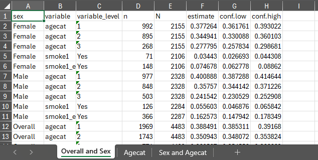
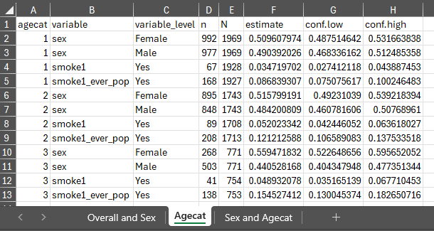
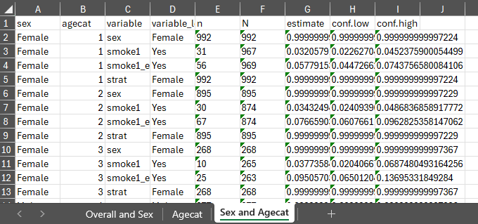
Exporting results and other outputs

Exporting results

With the previously generated results stored in results and results2 we can export the generated estimates to excel using export_results() and export_results2() in the respective stored tbl_svysummary objects.

export_results(results = results, file = "rw_results.xlsx")
export_results2(results = results2, file = "rw_results2.xlsx")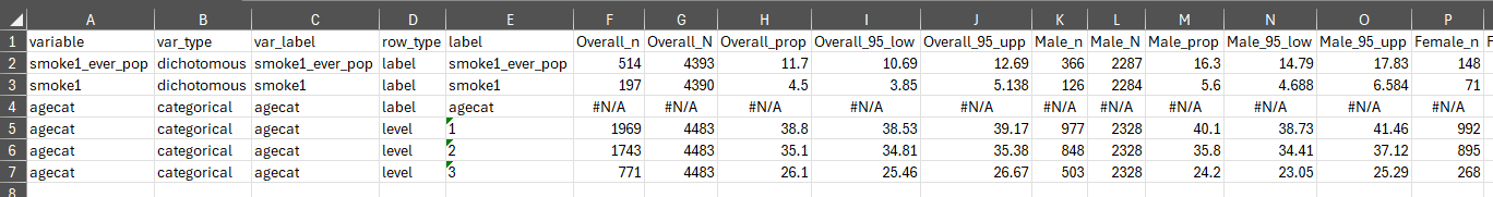

`export_results()` output:

`export_results2()` output:

Tab 1:

Tab 2:

Tab 3:

Visualizing questionnaire skip logic

The final function in the MPSurvey package is visualize_quex(). This function uses the questionnaire skip logic from the JSON file to create a directed graph showing the flow of questions and their skip patterns. You can also optionally include a value for responses to show the number of responses that flow in each pathway. This value can be directly used from the output of the get_inr() function by using inr$responses.

visualize_quex(path = "manifest.json",
               file = "rw_quex.pdf",
               responses = TRUE,
               analysis = rw_analysis)